Pandas is a great python library for data handling. It declares 2 main classes:
- Series – for one dimensional array
- DataFrame – for 2 dimensional tables (and with multi-indexing can display more dimensions)
Typical flow of using Pandas will be – load the data, manipulate and store again. This is very similar to SQL use with Select, Insert, Update and Delete statement
In this post i will cover the basic operations in pandas compared to SQL statements
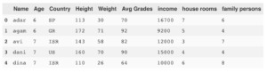
I will use a simple CSV file, load it to a dataframe and run all the commands on it:
import numpy as np
import pandas as pd

df=pd.read_csv('pupils.csv')
df.head()
Select
Select * from df where index between 2 and 6
df[2:6]
Select * from df where (index between 3 and 9) and (index % 2 = 1)
df[3:9:2]
Select Name from df
df['Name']
Select Name, Age from df
df[['Name','Age']]
Select Name where index between 2 and 6
df['Name'][2:6]
Select Name,Age where index between 2 and 6
df[['Name','Age']][2:6]
Note for reference – Same operations with loc:
df.loc[2] # index 2 as series
df.loc[2:2] # index 2 as dataframe
df.loc[2:6] # indexes 2-6
df.loc[2:6:2] # even indexes 2-6
df.loc[2:2]['Age'] # Age where index=2
df.loc[1,'Age'] # Age where index=1
df.loc[1:13:2,'Age':'income':2] # odd rows from 1 to 13 and even cols from Age to income
Same operations with iloc:
df.iloc[1] # where index=1
df.iloc[1,1] # Age where index=1
df.iloc[1:4] # where index between 1 and 3
df.iloc[1:4,2:4] # Country, Height where index between 1 and 3
Select * from df where Age > 12
df[df['Age']>10]
Select Name, Country from df where Age > 12
df[df['Age']>10][['Name','Country']]
Select * from df where Age>12 or Height > 130
df[(df['Age']>12) | (df['Height'] > 130)]
Select * from df where Age>12 and Height > 130
df[(df['Age']>12) & (df['Height'] > 130)]
Insert
Insert into df values (‘eli’,4,’DF’,100,20,20,2000,4,4)
df.loc[df.index.size]=['eli',4,'DF',100,20,20,2000,4,4]
Insert into df select * from df2
df.append(df2)
Insert new column with values (alter table df add Inc int; update df set Inc=income*2)
df['Inc']=df['income']*2
Update
Update df set Age=30
df.loc[:,'Age']=30
Update df set Age=20 where income>20000
df.loc[df['income']>20000,'Age']=20
Update df set income=income*2
df['income']*=2
Complex Update using iterator:
for i,v in df.iterrows():
    if v.Age > 10:
        df.loc[i,'Weight'] = 888
The above is a simple example but you can add as much logic as you need to the loop
Delete
Delete df where index=6
df.drop(6)
Delete df where Age=6
df.drop(df['Age']==6,inplace=True)
Delete column (alter table drop column Age)
df.drop('Age',axis=1)
Aggregates and Group By
Select count(*) from df
df.agg('count')
Select count(*),max(*) from df
df.agg(['count','max'])
Select count(Name), sum(income) , max(Age) from df
df.agg({'Name':'count', 'income':'sum' , 'Age':'max'})
select Country,count(*) from df group by Country
df.groupby('Country').count()
select Country,[family persons],count(*) from df group by Country,[family persons]
df1=df.groupby(['Country','family persons']).count()